Figure 16. The response in three different locations of the axon to a variable stimulus at x=0. Top panel: stimulus= 4uA, middle panel: stimulus=10 uA, bottom panel: stimulus=-10 uA.
Figure 16 shows the recording of the membrane potential in three different spots along a squid giant axon in response to several current stimuli at x=0. For a current pulse of 4 µA (top panel) the response is local and there is no detectable voltage changes at the second or third electrodes. For a pulse of 10 µA, there is a full action potential response in x=0 and also at x=2.5 and x=5 cm. The responses at 2.5 and 5 cm are similar in time course but delayed with respect to each other: these are recordings of the propagated action potential. A negative pulse of -10 µA produces only a local response in the negative direction and there is no propagation.
From the above, it is clear that the voltage is a complicated function of both time and distance, V=V(t,x). But, even worse, it is not a simple function of the stimulus, because there is little response for negative or small positive stimuli and a large voltage response (the action potential) for a larger pulse. This is an explosive process and the study of explosions is difficult unless we can control them.
The first simplification will be to eliminate propagation and this can be achieved in the squid giant axon by inserting a wire along the axis of the axon to make the inside isopotential. This is already an important simplification because with this operation we eliminate the x variable and now V is only function of time, V=V(t). What does the response look like when there is no propagation? In fact, it looks very much the same. Fig. 16 show the voltage responses (the Membrane action potential) to four different stimuli, two negative and two positive. The action potential response is only obtained for the large depolarization, as it was the case where propagation was allowed. Our conclusion is that the non-linear voltage response of the membrane to the current stimulus is an intrinsic property of the axon membrane.
Figure 17. The response of an axon with an axial wire to stimuli of -10, -4.5, 4.5 and 10 uA . Only the stimulus of 10 uA elicited an action potential.
Hodgkin and Huxley decided to study the properties of the axon membrane with voltage pulses instead of current pulses to control the explosive mechanism involved in the action potential generation. The technique used to deliver voltage pulses (or any other voltage waveform) to the membrane is called the voltage clamp and it was introduced by K. S. Cole.
We have learned that the Na and K channels in the axon change their open probability depending on the voltage across the membrane and in fact the Po is independent of the current flow. Therefore it is natural to study the properties of the membrane under voltage clamp instead of current stimulation because membrane potential is the variable that controls channel opening.
The second good reason to use voltage control is that the application of a sudden step of voltage will instantly charge the membrane capacitor, eliminating the contribution of the capacitive current in the recording of the membrane current(5).
We have studied the properties of single K and Na channels in response to voltage steps and our study was done under voltage clamp because we were imposing voltage steps with the patch pipette across the membrane. This is easily accomplished with the patch clamp technique because, as the pipette diameter is only 1-2 µm, the membrane potential is homogeneous in the patch.
A different situation arises if one wishes to study the properties of a population of channels in a large membrane area under voltage clamp, as it is the case of the axon. This is because imposing a voltage in one spot does not guarantee that other regions further away will have the same potential. In fact, as we will see later, the potential in other regions is different.
This problem has been solved in the case of the squid giant axon introducing a wire inside the axon (the black axial wire in Fig. 18) to make the interior of the axon isopotential as we did it before to eliminate propagation. The voltage clamp is achieved using a negative feedback arrangement that compares Vm=Vi-Ve with Vc, the command voltage, to inject the appropriate current I, which will be equal to the membrane current. Therefore, in this technique the experimenter imposes a membrane voltage Vc and measures the membrane current I.
Figure 19. Ionic currents in response to hyperpolarizing pulses from -70 to -120 mV in 10 mV increment.
Figure 20. Currents in response to depolarizing pulses from -60 to 60 mV in increment of 10 mV from a holding potential of -70 mV.
The membrane currents during voltage
clamp.
If we run a series of voltage steps starting from -70 mV (near the resting potential)
we find that for hyperpolarizing pulses (negative going, such as to -90 mV)
the membrane current is negative (inward current) as expected, and it grows
linearly with the magnitude of the step (see Fig. 19) . In addition, the current
through the membrane is practically constant in time, indicating that it behaves
close to a passive resistor. For depolarizing (positive going) pulses (see Fig.
20) the same is observed for only very small pulses but for larger depolarizations,
the current is much larger (compare the calibration bar in Figs. 19 and 20).
The current first is inwardly directed and later in the pulse
it becomes outward (see Fig. 20). The initial inward current
is maximum when the potential is about 0 mV and with larger depolarizations
becomes smaller. Beyond +40 mV the outward current exhibit a first fast component
and then a slower rising and maintained component.
We know from the results of single channel recordings that there are two main types of channels: Na and K. In the case of single channel recordings, the separation of the channels is relatively simple: if there is one channel in the patch, we just observe its characteristics and decide which type it is. When the recording is from a large region of membrane that may contain 10 billion channels, the recorded current will be the average contribution of both type of channels, and the actual current waveform will depend on the proportion of Na and K channels in the membrane. Hodgkin and Huxley separated the two components by changing the ionic composition of the solution bathing the axon (exchanging Na for an impermeant ion).
The giant axon can be internally perfused, allowing the exchange of the internal
medium to different solutions of known composition. We will describe now the
ionic currents of the axon by controlling the ionic composition on both sides
of the axon (Hodgkin and Huxley exchanged the external solution only); this
procedure will allow us to separate specific components of the ionic currents.
We will identify these currents with the currents produced by K and Na channels
whose properties have already been described at the single channel level. The
following sections will give an overview of the macroscopic currents, and they
will expand on some aspects that were not treated in detail in the sections
on single channel properties.
Figure 21. Family of potassium currents elicited by pulses from a holding potential of -70 to +60 mV in increments of 10 mV.
The Potassium current. We will start by exchanging all sodium ions on both sides of the membrane with the cation choline. This ion was found to be impermeant by Hodgkin and Katz and by Hodgkin and Huxley. In addition we will add a toxin called tetrodotoxin (TTX) which was found to block the sodium conductance. Under these conditions if we perform a voltage clamp experiment as described above, the currents are quite different (see Fig. 21). All the inward components as well as the early outward current have disappeared. The general characteristics of these currents are that they become larger and faster as the depolarization is increased and that they are absent for hyperpolarizing pulses. This is exactly what we found when we averaged many single K channel recordings at several potentials (see Figs. 10, 11 and 12). As expected, the current is outward with depolarization because the internal concentration of potassium is about 40 times the concentration of potassium outside. We can characterize this current by plotting the current at the end of the pulse as a function of the membrane potential during the pulse as shown by the open circles in Fig. 22. where it is clearly seen that the I vs. V relation is very non-linear for depolarizing pulses and practically zero for hyperpolarizing potentials. The open squares in Fig. 22 corresponds to the open channel characteristics scaled by the number of channels, and as expected, it is linear and crosses the axis at the potassium reversal potential (see Fig. 13).
If the potassium inside and outside the axon is replaced by choline, then most of the current disappears, suggesting strongly that it is carried by potassium; the current that remains is very small and is linearly related to voltage, that is, it behaves like a resistor This remaining current was called leakage by Hodgkin and Huxley and plays an important role in the resting potential and in the actual value of threshold for excitation.
The potassium conductance. Given the results of the previous paragraph it is possible to define a quantitative relationship between current and voltage using the concept of conductance. The current IK is given by the product of this conductance and the driving force:
IK=gK(V,t) (V-EK)
where gK(V,t) is a function of the potential V and time t.
The detailed analysis of the conductance will require the understanding of its time course and its dependence on voltage. If we take the potassium current traces and divide them by V-EK both during and after the pulse we have the time course of the conductance for that particular depolarization and its recovery upon repolarization. Examples of the time course of gK for two different depolarizations are shown in Fig. 23. The important features are:
i) the conductance develops faster at more positive potentials,
ii) the conductance at the end of a long pulse is larger at more positive potentials,
iii) the development of the conductance is sigmoid, that is, it shows a lag before turning on and upon repolarization it turns off without appreciable lag. These features are compatible with a high order process with multiple steps during turning on and a first order process in turning off.
Figure 23. The potassium conductance as a function of time during and after a pulse to -10 and 60 mV.
The correlation of the n formulation and single channels.
We have seen that the macroscopic ionic currents are the result of a large number
of unitary current events through single molecules called ionic channels. In
the simplified view of the K channel, the probability of the channel to be open,
Po, is given by n4
and the maximum conductance corresponds to the conductance of one channel
times all the channels available NK:
Then NK gK Po=gK(V,t) and NK gK= gKmax. As we saw before, the parameter n is the probability that a subunit is in the active position, therefore n is a function of voltage and time, n=n(V,t) and so will be n4.
It is important to note that this formulation is able to predict the lag in
the conductance turn on (that is, upon depolarization) because all four gating
subunits must be in the active position for conduction to occur. As this requires
the movement of four subunits it is a fourth order process. On the other hand,
the turn off (that is, the repolarization) depends on the return of only one
of the subunits which is a first order process.
The sodium conductance. If the axon is
perfused and bathed in solutions free of potassium ions, the current recorded
for clamp steps are quite different than in the normal solutions as it was shown
in Fig. 15. In this series of traces, the holding potential was -70 mV and pulses
ranged from -60 to +60 in steps of 10 mV. The currents are inward for small
depolarizations and they are not maintained for the duration of the pulse but
instead they decrease spontaneously and, as the depolarization is made larger,
the turn on and turn off becomes faster. The direction of the current reverses
at about 50 mV and this potential coincides with the sodium Nernst sodium potential,
as computed with the known concentrations of sodium inside and outside the fiber.
If we plot the maximum (peak) current as a function of pulse amplitude
we obtain the relation plotted as open circles in the top panel of Fig. 24.
Notice that the current is inward for all potentials negative of 50 mV and outward
when the potential
is more positive than 50 mV. In addition, from this plot it is very clear that
the slope of the I-V relation is negative for potentials more
negative than about 0 mV. A negative slope in the I-V curve means that
there is a negative resistance, that is, an element that instead of
dissipating energy it is in fact injecting energy in the system. This energy
can be traced to the Na driving force that is forcing sodium ions to flow along
their electrochemical gradient. The squares in the top panel of Fig. 24 correspond
to the open channel characteristics scaled by the number of channels
(that is, NNa iNa).
The bottom panel of Fig. 24 is a plot of the peak conductance as a function of membrane potential and it shows the typical sigmoid relation as it was seen for the K channel. This plot was obtained by dividing the peak current by V-ENa. (The reader may verify that it can also be obtained by dividing the peak current by the scaled open channel current).
Inactivation of the sodium conductance. When we studied the single Na channel, we remarked that one of the salient features of the sodium current is its decay during the pulse, a process that has been called inactivation. We are going to describe a few experiments that give more insight on the onset and recovery of inactivation.
Figure 25. The effect of a long prepulse from -90 to -30 mV on the sodium current elicited by a pulse to 0 mV.
Fig. 25 shows a series of sodium currents elicited by a double pulse experiment.
The first pulse is varied between -90 and -30 mV and the second pulse is always
to 0 mV. Notice that the first pulse elicits a Na current for depolarizations
to -50, -40 and -30 mV and that the amplitude of the current during the second
pulse depends on the potential during the first pulse. This result
is very important because it shows that the current at 0 mV is not always the
same but it depends on the previous history: the more depolarization in the
previous pulse, the less current elicited by the second pulse. If we plot the
normalized current during the second pulse as a function of the value of the
first pulse we find a sigmoid curve as shown in Fig. 26.
This curve has been called the h curve because the inactivation process
is controlled by the variable h and the subindex refers to the value
of the variable for a very long prepulse. The prepulse effect develops with
time; for very short prepulses no channels are inactivated but as the prepulse
is made longer the percentage of channels that become inactivated increases.
When the prepulse is very long, the effect on the current during the test pulse
corresponds to the result obtained in Fig. 25 and shown as h in Fig.
26.
Figure 27. Experiment to determine the time required at -70 mV to recover from inactivation (see text).
Recovery from inactivation. A depolarization opens Na channels and, if maintained, these channels inactivate. A valid question is, how long do we have to wait for the channels to be ready to conduct again? First, it is clear that if the depolarization is maintained, the channel will not conduct because inactivation will persist. We must repolarize the membrane to reset the initial conditions. Fig. 27 shows an experiment to explore the recovery from inactivation. The membrane was pulsed to 0 mV for 10 ms producing an inward Na current. Then the membrane was repolarized back to -70 mV for a variable period of time before pulsing again to 0 mV for a period of 2 ms. The figure shows all the trials superimposed with different recovery intervals at -70 mV. When the recovery interval was 1 ms, the Na current was very small (about a tenth of the current elicited by the first pulse). As the recovery time at -70 mV was prolonged, the peak inward Na current started to increase, reaching half of its original amplitude at about 7 ms and almost fully recovered at about 27 ms (the rightmost current trace shown in the Fig. 27). These results show us that to get all the Na current back we have to return the membrane to its resting value for a period of at least 10 ms. This will have important consequences in the recovery from the refractory period in the action potential.
The leakage current. In addition to the Na and K currents, there is a small current that has essentially a linear dependence on the membrane potential, behaving as a pure resistor with a reversal potential more positive than EK but more negative than ENa. This current was attributed to non-specific conductances, which grouped together compose the leakage conductance that can be written as
IL=gL(V-EL).
The equivalent circuit of the axon membrane includes ionic pathways and a capacitor (see Fig. 2). When the voltage is constant, the current through the capacitative pathway is zero because the capacitor has acquired the charge Q according to the relationship
Q=CV
We have not yet addressed the situation when V is changing because during voltage clamp pulses V is constant (except for the instant when V is stepped up or down). If we are to understand the operation of the axon, we need to consider the situation when V is changing in time because that is exactly what is happening during the action potential.
We must ask first, how does the capacitor acquire the charge Q when the potential is changing from 0 to V? The answer is by allowing a flow of charge (ions) towards the plates (the membrane surfaces) and this flow constitutes an electric current which we will call Ic. We can calculate this current easily if we remember that current is the flow of charge, or the amount
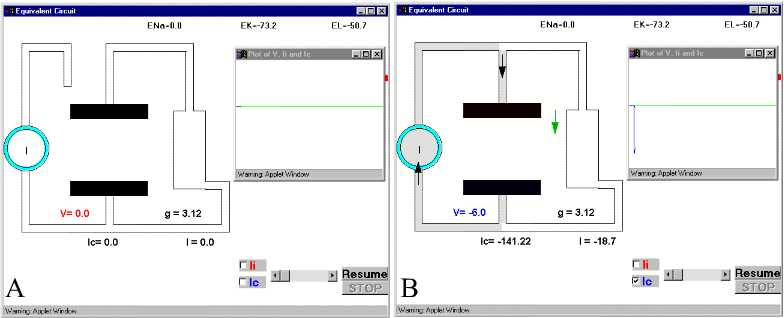
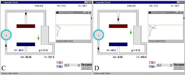
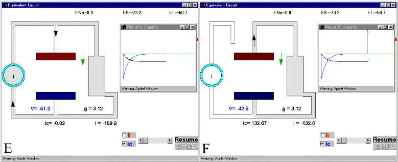
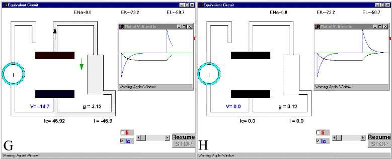
Figure 28. The charging and discharging of the membrane capacity. Ic and V are indicated in Panel D.For details see text. For simulation, press Simple RC after clicking here.
charges passing per unit time. In other words, Ic is the
first derivative of Q with respect to time

If we take the first derivative of Q=CV, we get

because C has been assumed to be a constant(6).
This equation tells us that as long as V is changing with time, there
will be a current flowing towards the capacitor. It also verifies that if V
is constant in time, there is no capacitive current.
To get a feeling of the importance of this capacitive current, look at the voltages and currents in the simple membrane circuit of Fig. 2 when we supply current with an external source. In Fig. 28 there is series of pictures that are snapshots of the current circulation in the resistive and capacitive branches after the current generator (the circle with the I inside) is connected and subsequently disconected. The intensity of the current is represented by the darkness in the wires. To the right of each panel, there is a plot of the membrane potential (which is the voltage across the capacitor) and the time course of the current in the capacitive branch.. This is the equivalent of connecting an stimulator and recording the voltage accross the membrane. To simplify the situation even more, let us assume that the membrane starts at 0 mV, that is, there is no internal battery. In Fig. 28A we have our equivalent circuit and a current generator that at present is disconnected from the membrane (the switch is open). The current generator will pass a constant amount of current I (which we will set as inward current) as soon as the switch is closed and the current will be distributed in the capacitative (Ic) and the resistive branch (the ionic channels Ii) as
I=Ic+Ii
In Fig 28B, we see how initially the current is going mainly into the capacitative branch with almost no current through resistive branch. (The downward spike in the plot corresponds to the capacitive current, which is negative because it is inward). It is clear that at very short times, most of the current supplied by the current generator will go into the capacitative branch because the capacitor was discharged, while the resistive branch will receive much less current.. Parts C and D and E of Fig. 28 show the current and voltage as time progresses. Notice that as the capacitive current subsides, the voltage builds up. At long times (part E), the capacitor has reached its full charge, V has leveled off to its maximum negative value, and consequently Ic becomes zero (Fig. 28 E). If at this point we open the switch, which is equivalent to stopping the current stimulus, then the capacitor will discharge through the resistor and the current in the capacitor branch will flow in the opposite direction. At short times the capacitive current will be very large because V is changing (Fig. 28F) and a large upward current spike reflects the discharging of the capacitor branch. As time goes on (Fig 28G and H) it will subside because all the charge has been redistributed and the energy has been dissipated as heat as the current circulates through the resistor.
The actual time course of the voltage across the membrane is given by solving the above equation of the total I after substituting Ii=V/R and Ic=CdV/dt. When the switch is closed, the result is
V=IR[1-exp(-t/tm)]
which is the exponential time course observed in Fig 28.
When we reopen the switch we get
V=-IR exp(-t/tm)
In both cases, the speed of charging depends on tm, which is the product of the membrane capacitance C and the membrane resistance R (tm=RC). This product tm has been called the membrane time constant. If R or C are small, the charging occurs very quickly, but on the contrary, if they are large, it takes more time to reach the final value.
GENERATION OF THE ACTION POTENTIAL
NOTES:
5. If the capacitor is ideal and there is no resistance in series, the application of a voltage V will produce an infinite amount of current in an infinitesimally short time transporting a charge q=CV. In practice V is not an step and there is a series resistance, therefore the capacitive current will last a finite time.
6. In the axon, part of the membrane capacitance is a function of voltage due to the gating mechanisms but it is a small fraction that has a negligible effect in the interpretation of the action potential generation